GDAS005-基因组实验中的数据结构与管理

前言

在科学研究中,大家都认为数据管理是一项专业且乏味的工作。因为数据管理一旦出现问题,会导致自身的资源与声誉付出高昂的代价,因此,数据管理必须要高度可靠且有效。在传统实验室中,研究人员通常使用电子表格来管理数据,但是这种方式存在着风险。因此,我们希望通常简化可靠的数据管理操作来增加数据的价值。

在Bioconductor中,指导软件开发的原则也可以应用于数据管理。模块化和可扩展的数据结构能够发挥更高的价值。打包和版本控制协议适用于定义数据类(data class)。我们可以将电子表格转化为语义丰富的对象,并联合使用NCBI GEO数据库,处理BAM和BED文件,以及外部存储来促进与大型多组学数据库(例如TCGA)衔接来说明一下上述的这些思路。

汇总多个表格信息

演示包:GSE5859Subset

GSE5859Subset是一个包,里面含有一个实验的表达数据。当加载了这个包后,我们可以看到这个包有三个组件:

1
2
3
4
5
6
7
8
library(GSE5859Subset)
data(GSE5859Subset)
dim(geneExpression)
## [1] 8793 24
dim(geneAnnotation)
## [1] 8793 4
dim(sampleInfo)
## [1] 24 4

我们来查看一下这3个组件是否有关(一个矩阵,两个数据框),如下所示:

1
2
3
4
all.equal(sampleInfo$filename, colnames(geneExpression))
## [1] TRUE
all.equal(rownames(geneExpression), geneAnnotation$PROBEID)
## [1] TRUE

简单来讲,我们可以把 sampleInfo$filename 视为一个按行连接的节点(key),它连接了样本信息表格与基因表达表格。colnames(geneExpression)将该矩阵的列连接到sampleInfo的行中对应的样本。简单来说就是,geneExpression的列名是样本名,而sampleInfo中的某1列中也含有这些样本名,如下所示:

与之类似, geneExpression 的行名,对应了geneAnnotation中探针数据,即 PROBEID ,如下所示:

1
2
3
4
5
6
7
8
9
10
11
options(digits=2)
cbind(sampleInfo[1:3,], colnames(geneExpression)[1:3],
t(geneExpression)[1:3,1:4])
## ethnicity date filename group
## 107 ASN 2005-06-23 GSM136508.CEL.gz 1
## 122 ASN 2005-06-27 GSM136530.CEL.gz 1
## 113 ASN 2005-06-27 GSM136517.CEL.gz 1
## colnames(geneExpression)[1:3] 1007_s_at 1053_at 117_at 121_at
## 107 GSM136508.CEL.gz 6.5 7.5 5.4 7.9
## 122 GSM136530.CEL.gz 6.4 7.3 5.1 7.7
## 113 GSM136517.CEL.gz 6.3 7.2 5.0 7.5

在ExpressionSet汇总表格

ExpressionSet 容器用于管理一个项目中的所有信息。为了改善基因名与样本名命名的可视化效果,我们可以以下每个组件的注释信息,如下所示:

1
2
3
4
5
6
head(rownames(sampleInfo))
head(rownames(geneAnnotation))
rownames(sampleInfo) = sampleInfo$filename
rownames(geneAnnotation) = geneAnnotation$PROBEID
head(rownames(sampleInfo))
head(rownames(geneAnnotation))

结果如下所:

1
2
3
4
5
6
7
8
9
10
11
12
> head(rownames(sampleInfo))
[1] "107" "122" "113" "163" "153" "161"
> head(rownames(geneAnnotation))
[1] "1" "30" "31" "32" "33" "34"
> rownames(sampleInfo) = sampleInfo$filename
> rownames(geneAnnotation) = geneAnnotation$PROBEID
> head(rownames(sampleInfo))
[1] "GSM136508.CEL.gz" "GSM136530.CEL.gz" "GSM136517.CEL.gz"
[4] "GSM136576.CEL.gz" "GSM136566.CEL.gz" "GSM136574.CEL.gz"
> head(rownames(geneAnnotation))
[1] "1007_s_at" "1053_at" "117_at" "121_at" "1255_g_at"
[6] "1294_at"

现在我们已经将样本的信息进行了更改,现在我们生成 ExpressionSet,如下所示:

1
2
3
4
5
6
7
8
9
10
11
12
13
14
15
16
17
18
19
20
21
library(Biobase)
es5859 = ExpressionSet(assayData=geneExpression)
pData(es5859) = sampleInfo
fData(es5859) = geneAnnotation
es5859
## ExpressionSet (storageMode: lockedEnvironment)
## assayData: 8793 features, 24 samples
## element names: exprs
## protocolData: none
## phenoData
## sampleNames: GSM136508.CEL.gz GSM136530.CEL.gz ...
## GSM136572.CEL.gz (24 total)
## varLabels: ethnicity date filename group
## varMetadata: labelDescription
## featureData
## featureNames: 1007_s_at 1053_at ... AFFX-r2-P1-cre-5_at (8793
## total)
## fvarLabels: PROBEID CHR CHRLOC SYMBOL
## fvarMetadata: labelDescription
## experimentData: use 'experimentData(object)'
## Annotation:

这样做的一个好处的就是,我们可以使用fDatapData组件中更高层次的注释来选择特征。例如,我们现在只提取Y染色体上的基因表达特征:

1
2
3
4
5
6
7
8
9
10
11
12
13
14
15
16
es5859[which(fData(es5859)$CHR=="chrY"),]
## ExpressionSet (storageMode: lockedEnvironment)
## assayData: 21 features, 24 samples
## element names: exprs
## protocolData: none
## phenoData
## sampleNames: GSM136508.CEL.gz GSM136530.CEL.gz ...
## GSM136572.CEL.gz (24 total)
## varLabels: ethnicity date filename group
## varMetadata: labelDescription
## featureData
## featureNames: 201909_at 204409_s_at ... 211149_at (21 total)
## fvarLabels: PROBEID CHR CHRLOC SYMBOL
## fvarMetadata: labelDescription
## experimentData: use 'experimentData(object)'
## Annotation:

我们可以看一下可ExpressionSet这种类所能使用的所有方法,如下所示:

1
2
3
4
5
6
7
8
9
10
11
12
13
14
15
16
17
18
19
20
methods(class="ExpressionSet")
## [1] [ [[ [[<- $$
## [5] $$<- abstract annotation annotation<-
## [9] as.data.frame as.matrix assayData assayData<-
## [13] boxplot classVersion classVersion<- coerce
## [17] combine description description<- dim
## [21] dimnames dimnames<- dims esApply
## [25] experimentData experimentData<- exprs exprs<-
## [29] fData fData<- featureData featureData<-
## [33] featureNames featureNames<- fvarLabels fvarLabels<-
## [37] fvarMetadata fvarMetadata<- initialize isCurrent
## [41] isVersioned KEGG2heatmap KEGGmnplot makeDataPackage
## [45] notes notes<- pData pData<-
## [49] phenoData phenoData<- preproc preproc<-
## [53] protocolData protocolData<- pubMedIds pubMedIds<-
## [57] rowMedians rowQ sampleNames sampleNames<-
## [61] show storageMode storageMode<- updateObject
## [65] updateObjectTo varLabels varLabels<- varMetadata
## [69] varMetadata<- write.exprs
## see '?methods' for accessing help and source code

在这些方法中比较重要的有以下几个:

  • exprs(): 获取数值型表达值;
  • pData(): 获取样本数据,就是样本名;
  • fData(): 获取特征数据,就是基因表达值;
  • annotation(): 获取特征名的标签;get a tag that identifies nomenclature for feature names
  • experimentData(): 获取符合 MIAME的元数据结构。

许多方法都具有setter属性(注:这里的setter应该是R面向对象编程中的一个方法,我猜测可能是赋值一类的操作,具体的我还不清楚)。例如,

exprs<- 可以用于指定表达数值。此外,所有的组件都是可选的,因此我们的es5859对象中没有annotationexperimentData也不奇怪。我们随后会改善一下这个对象的自身的描述,首选我们设置注释信息,如下所示:

1
2
3
annotation(es5859)
annotation(es5859) = "hgfocus.db" # need to look at GSE record in GEO, and know .db
annotation(es5859)

结果如下所示:

1
2
3
4
5
6
> annotation(es5859)
character(0)
> annotation(es5859) = "hgfocus.db" # need to look at GSE record in GEO, and know .db
>
> annotation(es5859)
[1] "hgfocus.db"

第二,获取符合MIAME文档的实验元数据信息,如下所示:

1
2
3
4
5
6
7
8
9
10
11
12
13
14
15
16
17
18
19
20
21
22
library(annotate)
es5859
mi = pmid2MIAME("17206142")
experimentData(es5859) = mi
es5859
## ExpressionSet (storageMode: lockedEnvironment)
## assayData: 8793 features, 24 samples
## element names: exprs
## protocolData: none
## phenoData
## sampleNames: GSM136508.CEL.gz GSM136530.CEL.gz ...
## GSM136572.CEL.gz (24 total)
## varLabels: ethnicity date filename group
## varMetadata: labelDescription
## featureData
## featureNames: 1007_s_at 1053_at ... AFFX-r2-P1-cre-5_at (8793
## total)
## fvarLabels: PROBEID CHR CHRLOC SYMBOL
## fvarMetadata: labelDescription
## experimentData: use 'experimentData(object)'
## pubMedIds: 17206142
## Annotation: hgfocus.db

现在我们通过abstract方法就能获取一定信息:

Now, for example, the abstract method will function well:

1
2
3
4
nchar(abstract(es5859))
## [1] 1057
substr(abstract(es5859),1,50)
## [1] "Variation in DNA sequence contributes to individua"

用于汇总这些表格的最新方法就是使用SummarizedExperiment类,我们后面会讲到。

*自同态环概念(endomorphism)

关于ExpressionSet容器设计的一个最后备注:假设 x 是一个ExpressionSet。方括号被定义为一操作符,当GS分别是标识特征和合适样本的合适向量时,那么X[G,S]是具有仅限于GS中标记的那些特征值和样本的ExrpessionSet。对X有限的所有操作也都对 X[G, S] 有效。此属性称为ExpressionSet相对于中括号进行子集的自同态。

上面一段不太懂,以下是原文:

A final remark about the ExpressionSet container design: Suppose X is an ExpressionSet. The bracket operator has been defined so that whenever G and S are suitable vectors identifying features and samples respectively, X[G, S] is an ExpressionSet with features and samples restricted to those identified in G and S. All operations that are valid for X are valid for X[G, S]. This property is called the endomorphism of ExpressionSet with respect to subsetting with bracket.

GEO, GEOquery, ArrayExpress与表达数据储存

基因表达数据库(GEO)储存了源于NIH资助的所有微阵列实验的数据。 Bioconductor的GEOquery软件包可以很方便地获取这些数据。而ArrayExpress软件包则可以很容易地获取欧洲分子生物学实验室赞助的ArrayExpress数据。

GEOmetadb

GEO中有数以万计的实验结果。GEOmetadb包括了用于获取和检索SQLite数据库的工具,SQLite数据库含有对GEO内容的广泛注释信息。2017年10月检索到的信息超过了6G。因此,我们并不需要你使用这个包。如果你有兴趣的话,可以参考vignette中案例,介绍得非常详细。

getGEO获取GEO中的ExpressionSet

例如我们对胶质母细胞瘤的基因组学特别感兴趣,并且已经性了一篇论文(Pmid 27746144)讨论了一种新陈代谢途径作可能会增强其治疗开发策略。这个实验使用了Affymetrix PrimeView阵列,并储存在GEO。现在我们使用getGEO获取这些数据,如下所示:

1
2
3
4
5
6
7
8
9
10
11
12
13
14
15
16
17
18
19
20
21
22
23
24
25
26
27
28
29
30
31
32
33
34
35
36
37
38
39
40
41
42
43
44
45
46
47
48
library(GEOquery)
glioMA = getGEO("GSE78703")[[1]]
## Found 1 file(s)
## GSE78703_series_matrix.txt.gz
## Parsed with column specification:
## cols(
## ID_REF = col_character(),
## GSM2072905 = col_double(),
## GSM2072906 = col_double(),
## GSM2072907 = col_double(),
## GSM2072908 = col_double(),
## GSM2072909 = col_double(),
## GSM2072910 = col_double(),
## GSM2072911 = col_double(),
## GSM2072912 = col_double(),
## GSM2072913 = col_double(),
## GSM2072914 = col_double(),
## GSM2072915 = col_double(),
## GSM2072916 = col_double()
## )
## File stored at:
## /var/folders/5_/14ld0y7s0vbg_z0g2c9l8v300000gr/T//RtmpKRbO0i/GPL15207.soft
## Warning: 102 parsing failures.
## row col expected actual file
## 49294 SPOT_ID 1/0/T/F/TRUE/FALSE AFFX-BioB-3_at literal data
## 49295 SPOT_ID 1/0/T/F/TRUE/FALSE AFFX-BioB-5_at literal data
## 49296 SPOT_ID 1/0/T/F/TRUE/FALSE AFFX-BioB-M_at literal data
## 49297 SPOT_ID 1/0/T/F/TRUE/FALSE AFFX-BioC-3_at literal data
## 49298 SPOT_ID 1/0/T/F/TRUE/FALSE AFFX-BioC-5_at literal data
## ..... ....... .................. .............. ............
## See problems(...) for more details.
glioMA
## ExpressionSet (storageMode: lockedEnvironment)
## assayData: 49395 features, 12 samples
## element names: exprs
## protocolData: none
## phenoData
## sampleNames: GSM2072905 GSM2072906 ... GSM2072916 (12 total)
## varLabels: title geo_accession ... treated with:ch1 (35 total)
## varMetadata: labelDescription
## featureData
## featureNames: 11715100_at 11715101_s_at ... AFFX-TrpnX-M_at
## (49395 total)
## fvarLabels: ID GeneChip Array ... SPOT_ID (36 total)
## fvarMetadata: Column Description labelDescription
## experimentData: use 'experimentData(object)'
## pubMedIds: 27746144
## Annotation: GPL15207

通过以上操作中,我们可以看到使用这个对象(数据集)可以查看使用LXR-623处理能够影响基因ABCA1的表达,文献对应的PubMed ID为27746144。

ArrayExpress检索并获取EMBL-EBI的ArrayExpress

ArrayExpress Archive of Functional Genomics Data储存了高通量功能基因组实验的数据,并为其他研究者再次使用这些数据提供方便。最近,ArrayExpress还从NCBI GEO导入了所有表达数据。

ArrayExpress包支持使用queryAE直接查询EMBL-EBI数据库,现在我们来试一下:

1
2
3
4
5
6
7
8
9
library(ArrayExpress)
sets = queryAE(keywords = "glioblastoma", species = "homo+sapiens")
dim(sets)
## [1] 546 8
sets[5:7,-c(7,8)]
## ID Raw Processed ReleaseDate PubmedID Species
## E-MTAB-6881 E-MTAB-6881 no no 2019-04-30 NA Homo sapiens
## E-MTAB-6882 E-MTAB-6882 no no 2019-04-29 NA Homo sapiens
## E-MTAB-7490 E-MTAB-7490 yes no 2019-03-22 NA Homo sapiens

PubmedID这一列显示的是Pubmed号,有的有,有的没有(没有的用NA标记),通过getAE函数则可以获取原始数据,如下所示:

1
2
initdir = dir()
if (!file.exists("E-MTAB-5797.sdrf.txt")) nano = getAE("E-MTAB-5797")

上面的代码将与该实验相关的数据下载到当前文件夹,如下所示:

1
2
3
4
5
6
7
8
9
afterget = dir()
setdiff(afterget, initdir)
## [1] "9406922003_R01C01_Grn.idat" "9406922003_R01C01_Red.idat"
## [3] "9406922003_R02C01_Grn.idat" "9406922003_R02C01_Red.idat"
## [5] "9406922003_R03C02_Grn.idat" "9406922003_R03C02_Red.idat"
## [7] "9406922003_R04C02_Grn.idat" "9406922003_R04C02_Red.idat"
## [9] "9406922003_R05C01_Grn.idat" "9406922003_R05C01_Red.idat"
## [11] "A-MEXP-2255.adf.txt" "E-MTAB-5797.idf.txt"
## [13] "E-MTAB-5797.raw.1.zip" "E-MTAB-5797.sdrf.txt"

在接下来的部分里,我们会讲解一下如何导入并处理这些数据。

SummarizedExperiment实例

在使用微阵列的时代,目标核酸的是由微阵列里面的探针决定的。而在现在广泛使用的短读长测序方法则为目标核酸的定量提供了更大的灵活性。因此,Bioconductor针对大规模的基因检测设计了一种更加灵活的容器。这种容器的一个重要思路就是我们仅仅通过基因组的坐标就能对我们的目标核酸进行识别。这种容器容器可以使用户们仅仅使用基因组坐标就能方便地分析各种数据。通用方法subsetByOverlaps可以与SummarizedExperiment实例配合使用来实现这一目标。

常规思路

应用于SummarizedExperiment的方法要比ExpressionSet的多,如下所示:

1
2
3
4
5
6
7
8
9
10
11
12
13
14
15
16
17
18
19
20
21
22
23
24
25
26
27
28
29
30
31
32
33
34
35
36
37
38
39
40
methods(class="SummarizedExperiment")
## [1] != [ [[
## [4] [[<- [<- %in%
## [7] < <= ==
## [10] > >= $$
## [13] $$<- aggregate anyDuplicated
## [16] anyNA append as.character
## [19] as.complex as.data.frame as.env
## [22] as.integer as.list as.logical
## [25] as.matrix as.numeric as.raw
## [28] assay assay<- assayNames
## [31] assayNames<- assays assays<-
## [34] bindROWS by c
## [37] cbind coerce coerce<-
## [40] colData colData<- countOverlaps
## [43] dim dimnames dimnames<-
## [46] duplicated elementMetadata elementMetadata<-
## [49] eval expand expand.grid
## [52] extractROWS FactorToClass findOverlaps
## [55] head intersect is.na
## [58] length lengths match
## [61] mcols mcols<- merge
## [64] mergeROWS metadata metadata<-
## [67] mstack names names<-
## [70] NROW overlapsAny parallelSlotNames
## [73] pcompare rank rbind
## [76] realize relist rename
## [79] rep rep.int replaceROWS
## [82] rev rowData rowData<-
## [85] ROWNAMES rowRanges rowRanges<-
## [88] selfmatch seqlevelsInUse setdiff
## [91] setequal shiftApply show
## [94] sort split split<-
## [97] subset subsetByOverlaps summary
## [100] table tail tapply
## [103] transform union unique
## [106] updateObject values values<-
## [109] window window<- with
## [112] xtabs xtfrm
## see '?methods' for accessing help and source code

不过其中的一些关键方法的使用类似于ExpressionSet中的方法,如下所示:

  • assay(): 获取原始数值量化结果,这里需要注意的是,该方法支持多个分析结果,使用assays()可以以列表的形式获取多个结果
  • colData(): 获取样本信息(从名字上来看,就是列信息)。
  • rowData(): 获取表达值信息。当表达值信息是使用基因组坐标来表示时,则可以使用 rowRanges()
  • metadata(): 获取可能包含相关实验的任何相关元数据的列表。

RNA-seq实验

现在我们使用 airway 包来演示一下 SummarizedExperiment的概念,如下所示:

1
2
3
4
5
6
7
8
9
10
11
library(airway)
data(airway)
airway
## class: RangedSummarizedExperiment
## dim: 64102 8
## metadata(1): ''
## assays(1): counts
## rownames(64102): ENSG00000000003 ENSG00000000005 ... LRG_98 LRG_99
## rowData names(0):
## colnames(8): SRR1039508 SRR1039509 ... SRR1039520 SRR1039521
## colData names(9): SampleName cell ... Sample BioSample

元数据(Metadata)是以列表的形式储存的,如下所示:

1
2
3
4
5
6
7
8
9
10
11
metadata(airway)
## [[1]]
## Experiment data
## Experimenter name: Himes BE
## Laboratory: NA
## Contact information:
## Title: RNA-Seq transcriptome profiling identifies CRISPLD2 as a glucocorticoid responsive gene that modulates cytokine function in airway smooth muscle cells.
## URL: http://www.ncbi.nlm.nih.gov/pubmed/24926665
## PMIDs: 24926665
##
## Abstract: A 226 word abstract is available. Use 'abstract' method.

这个数据集中的表达矩阵有64102行,它们的使用ENSEMBL数据库的命名方法定量了外显子的表达量,如下所示:

1
2
3
4
5
6
7
8
9
10
11
12
13
14
15
16
17
18
19
20
21
22
rowRanges(airway)
## GRangesList object of length 64102:
## $$ENSG00000000003
## GRanges object with 17 ranges and 2 metadata columns:
## seqnames ranges strand | exon_id exon_name
## <Rle> <IRanges> <Rle> | <integer> <character>
## [1] X 99883667-99884983 - | 667145 ENSE00001459322
## [2] X 99885756-99885863 - | 667146 ENSE00000868868
## [3] X 99887482-99887565 - | 667147 ENSE00000401072
## [4] X 99887538-99887565 - | 667148 ENSE00001849132
## [5] X 99888402-99888536 - | 667149 ENSE00003554016
## ... ... ... ... . ... ...
## [13] X 99890555-99890743 - | 667156 ENSE00003512331
## [14] X 99891188-99891686 - | 667158 ENSE00001886883
## [15] X 99891605-99891803 - | 667159 ENSE00001855382
## [16] X 99891790-99892101 - | 667160 ENSE00001863395
## [17] X 99894942-99894988 - | 667161 ENSE00001828996
## -------
## seqinfo: 722 sequences (1 circular) from an unspecified genome
##
## ...
## <64101 more elements>

在以前使用微阵列的时候,我们可能习惯于基因水平的定量信息。但在这个案例中,我们使用的外显子水平的定量信息,因此这里需要一个特定的计算方法将其转换为基因的定量信息。例如,基因ORMDL3在ENSEMBL中的标记符为ENSG00000172057,那么在SummarizedExperiment对象中,它所对应的坐标如下所示:

1
2
3
4
5
6
7
8
9
10
11
12
13
14
15
16
17
rowRanges(airway)$ENSG00000172057
## GRanges object with 20 ranges and 2 metadata columns:
## seqnames ranges strand | exon_id exon_name
## <Rle> <IRanges> <Rle> | <integer> <character>
## [1] 17 38077294-38078938 - | 549057 ENSE00001316037
## [2] 17 38077296-38077570 - | 549058 ENSE00002684279
## [3] 17 38077929-38078002 - | 549059 ENSE00002697088
## [4] 17 38078351-38078552 - | 549060 ENSE00002718599
## [5] 17 38078530-38078938 - | 549061 ENSE00001517665
## ... ... ... ... . ... ...
## [16] 17 38081876-38083094 - | 549072 ENSE00001517669
## [17] 17 38082049-38082592 - | 549073 ENSE00002700064
## [18] 17 38083070-38083099 - | 549074 ENSE00002688012
## [19] 17 38083320-38083482 - | 549075 ENSE00002700595
## [20] 17 38083737-38083854 - | 549076 ENSE00001283878
## -------
## seqinfo: 722 sequences (1 circular) from an unspecified genome

另外,GenomicRanges的工作类似于rowRanges() 。 如果要查看在这个列表中外显子坐标是否存在重叠区域,可以使用 reduce()方法,如下所示:

1
2
3
4
5
6
7
8
9
10
11
12
13
14
reduce(rowRanges(airway)$ENSG00000172057)
## GRanges object with 8 ranges and 0 metadata columns:
## seqnames ranges strand
## <Rle> <IRanges> <Rle>
## [1] 17 38077294-38078938 -
## [2] 17 38079365-38079516 -
## [3] 17 38080283-38080478 -
## [4] 17 38081008-38081058 -
## [5] 17 38081422-38081624 -
## [6] 17 38081876-38083099 -
## [7] 17 38083320-38083482 -
## [8] 17 38083737-38083854 -
## -------
## seqinfo: 722 sequences (1 circular) from an unspecified genome

这表明从外显子集合投身到基因组中的信息有可能包含8个被转录的亚区域。关于如何将这些信息转换为基因水平的定量信息,可以参考其它章节 elsewhere in the genomicsclass book.

除了对表达值进行详细地注释外,我们还需要colData()来处理样本信息。其中 $ 符号可以从列中提取样本信息,如下所示:

1
2
3
4
5
6
7
names(colData(airway))
## [1] "SampleName" "cell" "dex" "albut" "Run"
## [6] "avgLength" "Experiment" "Sample" "BioSample"
table(airway$dex) # main treatment factor
##
## trt untrt
## 4 4

处理由Illumina 450k甲基化芯片生成的数据

SummarizedExperiment 类设计出来用于储存所有类似的芯片数据或短序列读长测序数据。前面我们提到的 getAE 用于从ArrayExpress提取了一批文件,这批文件是胶质母细胞瘤组织中的甲基化定量数据。

而样本信息储存在 sdrf.txt 文件中,如下所示:

1
2
3
4
5
6
7
8
9
10
library(data.table)
sd5797 = fread("E-MTAB-5797.sdrf.txt")
head(sd5797[,c(3,16,18)])
## Characteristics[age] Label Performer
## 1: 58 Cy3 IntegraGen SA, Evry, France
## 2: 58 Cy5 IntegraGen SA, Evry, France
## 3: 72 Cy3 IntegraGen SA, Evry, France
## 4: 72 Cy5 IntegraGen SA, Evry, France
## 5: 70 Cy3 IntegraGen SA, Evry, France
## 6: 70 Cy5 IntegraGen SA, Evry, France

原始表达数据储存在 idat 文件中。现在我们使用 mnfi 包中的read.metharray() 函数将其提取出来,如下所示:

1
2
3
4
5
6
7
8
9
10
11
12
13
14
15
16
library(minfi)
pref = unique(substr(dir(patt="idat"),1,17)) # find the prefix strings
raw = read.metharray(pref)
raw
## class: RGChannelSet
## dim: 622399 5
## metadata(0):
## assays(2): Green Red
## rownames(622399): 10600313 10600322 ... 74810490 74810492
## rowData names(0):
## colnames(5): 9406922003_R01C01 9406922003_R02C01 9406922003_R03C02
## 9406922003_R04C02 9406922003_R05C01
## colData names(0):
## Annotation
## array: IlluminaHumanMethylation450k
## annotation: ilmn12.hg19

现在已经出现了很多算法可以将原始数值转换为生物学上可以解释的相对甲基化数值。在这个案例中我们使用分位数归一化算法(quantile normalization)来将红色和绿色的信号转换为相对甲基化数值(M),并且估计SummarizedExperiment 实例中的拷贝数(CN, copy number),如下所示:

1
2
3
4
5
6
7
8
9
10
11
12
13
14
15
16
17
18
19
20
21
22
23
24
glioMeth = preprocessQuantile(raw) # generate SummarizedExperiment
# Require IlluminaHumanMethylation450kmanifest packages
# BiocManager::install("IlluminaHumanMethylation450kmanifest")
# BiocManager::install("IlluminaHumanMethylation450kanno.ilmn12.hg19")
## [preprocessQuantile] Mapping to genome.
## [preprocessQuantile] Fixing outliers.
## [preprocessQuantile] Quantile normalizing.
glioMeth
## class: GenomicRatioSet
## dim: 485512 5
## metadata(0):
## assays(2): M CN
## rownames(485512): cg13869341 cg14008030 ... cg08265308 cg14273923
## rowData names(0):
## colnames(5): 9406922003_R01C01 9406922003_R02C01 9406922003_R03C02
## 9406922003_R04C02 9406922003_R05C01
## colData names(3): xMed yMed predictedSex
## Annotation
## array: IlluminaHumanMethylation450k
## annotation: ilmn12.hg19
## Preprocessing
## Method: Raw (no normalization or bg correction)
## minfi version: 1.31.1
## Manifest version: 0.4.0

在后面部分中,我们会来讲解一下如何处理这些数据。

外部数据储存—HDF5Array, saveHDF5SummarizedExperiment

测试内存占用

在常规的交互式使用中,R数据都是驻留在内存中。我们可以使用 gc()函数来估计一下某个任务占用的内存。Ncell所占用的空间用于处理语言结构,例如解析树(parse tree)和名称空间(namespaces),Vcell的空间用于储存会话中加载的数字和字符数据,现在我们打开R,查看一下,如下所示:

专用于Ncell的空间用于处理语言结构,如解析树和名称空间,而专用于Vcell的空间用于存储会话中加载的数字和字符数据。在我的MacBook Air上,R的香草启动收益率

Space devoted to Ncells is used to deal with language constructs such as parse trees and namespaces, while space devoted to Vcells is used to store numerical and character data loaded in the session. On my macbook air, a vanilla startup of R yields

1
2
3
4
> gc()
used (Mb) gc trigger (Mb) max used (Mb)
Ncells 10410962 556.1 18810631 1004.6 16638654 888.6
Vcells 38615493 294.7 128861398 983.2 128847953 983.1

当我们加载了 airway 包后,再查看一下,如下所示:

1
2
3
4
5
> suppressMessages({library(airway)})
> gc()
used (Mb) gc trigger (Mb) max used (Mb)
Ncells 10410859 556.0 18810631 1004.6 16638654 888.6
Vcells 38613228 294.6 128861398 983.2 128847953 983.1

现在加载 airway 这个 SummarizedExperiment实例,如下所示:

1
2
3
4
5
6
7
> data(airway)
> gc()
used (Mb) gc trigger (Mb) max used (Mb)
Ncells 11229539 599.8 18810631 1004.6 16638654 888.6
Vcells 42534679 324.6 128861398 983.2 128847953 983.1
> dim(airway)
[1] 64102 8

随着加载数据的增多,内存的占用也在增大。使用 rm() 函数可以清除一些不使用的对象,从而释放内存,不过在实际分析过程中很少这样做,或者说这样做效率并不高。

HDF5用于外部存储

HDF5 的全称是Hierarchical Data Format Version 5,即层次性数据格式第五版,它是一种广泛用于储存数值型的数据结构,并且提供了各种科学编程语言的接口。HDF5Array 包简化了管理大量数据型数组的操作,它的使用如下所示:

1
2
3
4
5
6
library(airway)
library(HDF5Array) # setup for external serialization
## Loading required package: rhdf5
data(airway)
airass = assay(airway) # obtain numerical data, then save as HDF5
href = writeHDF5Array(airass, "airass.h5", "airway")

现在我们可以发现,当我们访问相同的数值型数据时,内存的占用并没有增长,如下所示:

1
2
3
4
5
6
7
8
9
10
11
> gc() # after attaching HDF5Array package
used (Mb) gc trigger (Mb) max used (Mb)
Ncells 11246377 600.7 18810631 1004.6 16638654 888.6
Vcells 42828456 326.8 128861398 983.2 128847953 983.1
> myd = HDF5Array("airass.h5", "airway") # get reference to data
> gc()
used (Mb) gc trigger (Mb) max used (Mb)
Ncells 11246488 600.7 18810631 1004.6 16638654 888.6
Vcells 42828777 326.8 128861398 983.2 128847953 983.1
> dim(myd)
[1] 64102 8

这样运行起来一切还都正常,不过我们更常用 SummarizedExperiment 容器来操作airway数据,也就是我们下面要讲解的内容。

SummarizedExperiment支持HDF5

针对某个特定的 SummarizedExperiment 实例,saveHDF5SummarizedExperiment能将数据与元素数据汇集在一起,控制内存占用,同时保留容器中丰度的信息,如下所示:

1
2
3
4
5
6
7
8
9
10
11
12
13
14
15
16
17
saveHDF5SummarizedExperiment(airway, "externalAirway", replace=TRUE)
newse = loadHDF5SummarizedExperiment("externalAirway")
newse
## class: RangedSummarizedExperiment
## dim: 64102 8
## metadata(1): ''
## assays(1): counts
## rownames(64102): ENSG00000000003 ENSG00000000005 ... LRG_98 LRG_99
## rowData names(0):
## colnames(8): SRR1039508 SRR1039509 ... SRR1039520 SRR1039521
## colData names(9): SampleName cell ... Sample BioSample
assay(newse[c("ENSG00000000005", "LRG_99"),
which(newse$dex == "trt")]) # use familiar subsetting
## <2 x 4> DelayedMatrix object of type "integer":
## SRR1039509 SRR1039513 SRR1039517 SRR1039521
## ENSG00000000005 0 0 0 0
## LRG_99 0 0 0 0

在这个案例中,处理SummarizedExperiment元数据的操作抵抗了外部化这些数据的优势,如下所示:

1
2
3
4
5
6
7
8
9
10
11
12
13
> gc() # after loading SummarizedExperiment
used (Mb) gc trigger (Mb) max used (Mb)
Ncells 11252592 601.0 18810631 1004.6 16638654 888.6
Vcells 42840344 326.9 128861398 983.2 128847953 983.1
> gc() # after loading SummarizedExperiment
used (Mb) gc trigger (Mb) max used (Mb)
Ncells 11252592 601.0 18810631 1004.6 16638654 888.6
Vcells 42840344 326.9 128861398 983.2 128847953 983.1
> newse = loadHDF5SummarizedExperiment("externalAirway")
> gc()
used (Mb) gc trigger (Mb) max used (Mb)
Ncells 11252922 601.0 18810631 1004.6 16638654 888.6
Vcells 44883257 342.5 128861398 983.2 128847953 983.1

对那些大量的数据,支持HDF5的SummarizedExperiment会在内存不够的情况下,提供灵活的计算。

GenomicFiles某个特定类型的文件家族

GenomicFiles 是一个用于管理文件集合的包。当我们不想整体对某批数据进行解析和建模时,这个包就比较重要了,它可以导入某些文件的部分内容。

GenomicFiles 类的实例有rowRangescolData 方法。我们可以在 GenomicFiles 实例的 colData 组件中提取有关样本或实验的元数据,并且可以使用 rowRanges 组件来查看感兴趣的基因组间隔信息。

BAM 文件集

现在我们使用一个案例来说明一下这个文件集。我们所使用的案例是由 Zarnack团队在2013年进行的一个HNRNPC敲除后的RNA-seq测序项目。在这个项目中,一共有8个Hela细胞样本,其中4个是野生型,4个使用了RNAi敲低了HNRNPC,这个基因位于14号染色体上。

RNAseqData.HNRNPC.bam.chr14 中已经包含了比对好的读长。BAM文件被储存在了一个名为 RNAseqData.HNRNPC.bam.chr14_BAMFILES 的向量中,如下所示:

1
2
3
4
5
6
7
library(RNAseqData.HNRNPC.bam.chr14)
library(GenomicFiles)
gf = GenomicFiles(files=RNAseqData.HNRNPC.bam.chr14_BAMFILES)
gf
## GenomicFiles object with 0 ranges and 8 files:
## files: ERR127306_chr14.bam, ERR127307_chr14.bam, ..., ERR127304_chr14.bam, ERR127305_chr14.bam
## detail: use files(), rowRanges(), colData(), ...

我们可以通过将感兴趣的区域绑定到对象中,从而增强一个文件的信息,现在我们使用 GRanges 来检索HNRNPC,如下所示:

1
2
hn = GRanges("chr14", IRanges(21677296, 21737638), strand="-")
rowRanges(gf) = hn

如果要提取与感兴趣的区域重叠的比对信息(alignments),我们可以使用GenomicFiles包中的 reduceByRange 方法。我们需要定义一个映射函数来加入到 reduceByRange 函数中。这个映射函数我们在下面会定义为 MAP() , 它的参数有两个,其中 r 表示感兴趣的范围,f 指的是,被解析的文件中比对信息的重叠范围。在MAP() 函数中我们还使用了 readGAlignmentPairs 函数,这是因为我们霜肆处理配对的末端测序数据,如下所示:

1
2
3
4
5
6
7
8
9
10
11
library(GenomicAlignments)
MAP = function(r, f)
readGAlignmentPairs(f, param=ScanBamParam(which=r))
ali = reduceByRange(gf, MAP=MAP)
## Warning in .make_GAlignmentPairs_from_GAlignments(gal, strandMode = strandMode, : 4 alignments with ambiguous pairing were dumped.
## Use 'getDumpedAlignments()' to retrieve them from the dump environment.
sapply(ali[[1]], length)
## ERR127306 ERR127307 ERR127308 ERR127309 ERR127302 ERR127303 ERR127304
## 2711 3160 2946 2779 86 98 158
## ERR127305
## 141

在这个案例中,我们大致比较了一下这8个样本的目标范围,对于前4个样本来说,有更多的读长与HNRNPC区域比对上了,因此我们可以知道前4个样本是野生型细胞,后4个样本有较少的读长与HNRNPC区域比对上,这表明它们是敲低的HNRNPC。这里我们注意的是,敲低的效率并不是100%的,也就是说,我们仍然有可能会检测到有HNRNPC的一些转录本。

BED 文件集

erma 这个包设计用来演示在内存不足的情况下,基于表观遗传学中各种细胞类型数据分析,如何打包大量的数据。 这个包创建的基础容器是对 GenomicFiles 的简单扩展,它使用 makeErmaSet() 函数进行构建,如下所示:

1
2
3
4
5
6
7
8
library(erma)
erset = makeErmaSet()
## NOTE: input data had non-ASCII characters replaced by ' '.
erset
## ErmaSet object with 0 ranges and 31 files:
## files: E002_25_imputed12marks_mnemonics.bed.gz, E003_25_imputed12marks_mnemonics.bed.gz, ..., E088_25_imputed12marks_mnemonics.bed.gz, E096_25_imputed12marks_mnemonics.bed.gz
## detail: use files(), rowRanges(), colData(), ...
## cellTypes() for type names; data(short_celltype) for abbr.

我们可以使用 colData 来查看样本信息,如下所示:

1
2
3
4
5
6
7
8
9
10
11
12
13
14
15
16
17
18
19
20
21
22
23
24
25
26
27
28
29
colData(erset)
## (showing narrow slice of 31 x 95 DataFrame) narrDF with 31 rows and 6 columns
## Epigenome.ID..EID. GROUP Epigenome.Mnemonic ANATOMY
## <character> <character> <character> <character>
## E002 E002 ESC ESC.WA7 ESC
## E003 E003 ESC ESC.H1 ESC
## E021 E021 iPSC IPSC.DF.6.9 IPSC
## E032 E032 HSC & B-cell BLD.CD19.PPC BLOOD
## E033 E033 Blood & T-cell BLD.CD3.CPC BLOOD
## ... ... ... ... ...
## E071 E071 Brain BRN.HIPP.MID BRAIN
## E072 E072 Brain BRN.INF.TMP BRAIN
## E073 E073 Brain BRN.DL.PRFRNTL.CRTX BRAIN
## E088 E088 Other LNG.FET LUNG
## E096 E096 Other LNG LUNG
## TYPE SEX
## <character> <character>
## E002 PrimaryCulture Female
## E003 PrimaryCulture Male
## E021 PrimaryCulture Male
## E032 PrimaryCell Male
## E033 PrimaryCell Unknown
## ... ... ...
## E071 PrimaryTissue Male
## E072 PrimaryTissue Mixed
## E073 PrimaryTissue Mixed
## E088 PrimaryTissue Female/Unknown
## E096 PrimaryTissue Female
## use colnames() for full set of metadata attributes.

我们可以使用熟悉的简捷方式来查看样本元数据的表格信息:

1
2
3
4
5
6
table(erset$ANATOMY)
##
## BLOOD BRAIN ESC FAT IPSC LIVER LUNG SKIN
## 15 7 2 1 1 1 2 1
## VASCULAR
## 1

因此我们可以在R中通过轻量级的接口(仅限于关于示例和文件路径的元数据)来访问大量的BED文件集。如果这些文件是用tabix建立索引的,那么我们就可以非常快速地针对性地检索特定范围的数据,我们可以使用 stateProfile 函数来说明这一点,如下所示:

注:tabix是第一个能够对排序好的TAB分割数据进行处理,例如GEF,BED,PSL,SAM与SQL的输出数据等,它能快速地检索特定区域的重合部分。具体的使用方法可以参考本文的参考资料。

1
2
3
4
stateProfile(erset[,26:31], shortCellType=FALSE)
## 'select()' returned 1:many mapping between keys and columns
## Scale for 'y' is already present. Adding another scale for 'y', which
## will replace the existing scale.

plot of chunk lkstpr

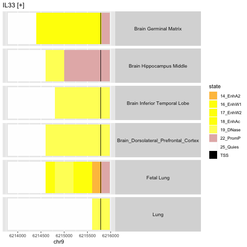
这张图描述在chr9的正义链上,基因IL33的启动子区域的表观遗传状态中的的解剖位点之间的变异。需要注意的是,胎儿肺样本似乎说明,与成人肺样本在这个区域的静默相比,胎儿肺样本则表现出增强子活性。。

管理大量的DNA变异信息

VCF背景

处理大量SNP基因型(或小indels)的最常用方法就是处理VCF文件(Variant Call Format)。从Wikipedia或相关文档,例如specdiagram很容易查看VCF文件的内容。VCF文件的基本设计中含有一个头部信息,这个头部信息提供了关于VCF文件的元数据,并且包括了每个基因组的突变体(variant)信息。这些突变体信息记录了突变体的性质(那些已经检测出来与参考基因组的差异信息),以及包括用于描述存在于突变体结构(variant configuration)中的样本字段(field)。一些突变体是已经确定的,而一些突变体则无法确定,在这种情况下,基因型的可能性就会被记录下来。突变体也许是阶段性的(phased),这就意味着,在某条具体的染色体上,突变的位置也有可能不同。

后两句话不太理解,这里放上原文:Some variants are “called”, others may be uncertain and in this case genotype likelihoods are recorded. Variants may also be phased, meaning that it is possible to locate different variant events on a given chromosome.

VariantAnnotation 包定义了处理这种格式的基础工具。Rsamtools 包有一个处理这些文件的tabix索引程序,因此也可以使用这个包。

*1000基因组VCF

DNA突变体的一个明显案例就是1000 genomes project。Bioconductr的 ldblock 包中有一个工具可以处理VCF文件,它能处理压缩的,由tabix建立索引的VCF文件,这个项目位于Amzon的云上,操作如下所示:

1
2
3
4
5
6
library(ldblock)
sta = stack1kg()
sta
## VcfStack object with 22 files and 2548 samples
## Seqinfo object with 22 sequences from an unspecified genome; no seqlengths
## use 'readVcfStack()' to extract VariantAnnotation VCF.

这里注意一下,创建的基因组标记为b37。这是一个不太寻常的特征,它绑定到了VCF突变体数据中的元数据里,无法被改变。

我们将在此文件中添加有关样本地理来源的信息。正好 ph525x 这个包中就包含这些地理信息,如下所示:

1
2
3
4
5
library(ph525x)
data(sampInfo_1kg)
rownames(sampInfo_1kg) = sampInfo_1kg[,1]
cd = sampInfo_1kg[ colnames(sta), ]
colData(sta) = DataFrame(cd)

注:这一部分的代码运行出错,经检索后,可能是由于网络问题。

输入并处理VCF数据

现在我们使用 GenomicFiles 包中的 readVcfStack 函数来提取VCF中的储存的内容。我们提取的内容是针对ORMDL3的编码区,如下所示:

1
2
3
4
5
6
7
8
9
10
11
12
13
14
15
16
17
18
19
20
21
22
23
24
25
26
27
28
29
30
31
32
library(erma)
orm = range(genemodel("ORMDL3")) # quick lookup
## 'select()' returned 1:many mapping between keys and columns
genome(orm) = "b37" # must agree with VCF
seqlevelsStyle(orm) = "NCBI" # use integer chromosome codes
ormRead = readVcfStack(sta, orm)
ormRead
## class: CollapsedVCF
## dim: 3 2548
## rowRanges(vcf):
## GRanges with 5 metadata columns: paramRangeID, REF, ALT, QUAL, FILTER
## info(vcf):
## DataFrame with 12 columns: AF, AC, NS, AN, EAS_AF, EUR_AF, AFR_AF, AM...
## info(header(vcf)):
## Number Type Description
## AF A Float Estimated allele frequency in the range (0,1)
## AC A Integer Total number of alternate alleles in called...
## NS 1 Integer Number of samples with data
## AN 1 Integer Total number of alleles in called genotypes
## EAS_AF A Float Allele frequency in the EAS populations cal...
## EUR_AF A Float Allele frequency in the EUR populations cal...
## AFR_AF A Float Allele frequency in the AFR populations cal...
## AMR_AF A Float Allele frequency in the AMR populations cal...
## SAS_AF A Float Allele frequency in the SAS populations cal...
## VT . String indicates what type of variant the line rep...
## EX_TARGET 0 Flag indicates whether a variant is within the e...
## DP 1 Integer Approximate read depth; some reads may have...
## geno(vcf):
## SimpleList of length 1: GT
## geno(header(vcf)):
## Number Type Description
## GT 1 String Phased Genotype

CollapsedVCF 类用于管理输入的基因型数据。现在我们检索3个突变体的信息。我们将得到的结果的子集转换为 VariantTools 所代表的VRanges 形式,从而可以更加清楚地了解到内容,如下所示:

1
2
3
4
5
6
7
8
9
10
11
12
13
14
15
16
17
18
19
20
21
22
23
24
25
26
27
28
29
30
31
32
33
34
35
36
37
38
39
40
41
42
library(VariantTools)
vr = as(ormRead[,1:5], "VRanges")
vr[1:3,]
## VRanges object with 3 ranges and 14 metadata columns:
## seqnames ranges strand ref
## <Rle> <IRanges> <Rle> <character>
## 17:38078372_T/TG 17 38078372 * T
## 17:38078393_TGG/T 17 38078393-38078395 * TGG
## 17:38078398_G/GGT 17 38078398 * G
## alt totalDepth refDepth
## <characterOrRle> <integerOrRle> <integerOrRle>
## 17:38078372_T/TG TG <NA> <NA>
## 17:38078393_TGG/T T <NA> <NA>
## 17:38078398_G/GGT GGT <NA> <NA>
## altDepth sampleNames softFilterMatrix |
## <integerOrRle> <factorOrRle> <matrix> |
## 17:38078372_T/TG <NA> HG00096 |
## 17:38078393_TGG/T <NA> HG00096 |
## 17:38078398_G/GGT <NA> HG00096 |
## QUAL AF AC NS
## <numeric> <NumericList> <IntegerList> <integer>
## 17:38078372_T/TG <NA> 0.01 61 2548
## 17:38078393_TGG/T <NA> 0.04 191 2548
## 17:38078398_G/GGT <NA> 0.05 272 2548
## AN EAS_AF EUR_AF AFR_AF
## <integer> <NumericList> <NumericList> <NumericList>
## 17:38078372_T/TG 5096 0 0 0.04
## 17:38078393_TGG/T 5096 0 0.01 0.13
## 17:38078398_G/GGT 5096 0.01 0.04 0.13
## AMR_AF SAS_AF VT EX_TARGET
## <NumericList> <NumericList> <CharacterList> <logical>
## 17:38078372_T/TG 0 0 INDEL FALSE
## 17:38078393_TGG/T 0.01 0.01 INDEL FALSE
## 17:38078398_G/GGT 0.02 0.03 INDEL FALSE
## DP GT
## <integer> <character>
## 17:38078372_T/TG 240289 0|0
## 17:38078393_TGG/T 222931 0|0
## 17:38078398_G/GGT 218409 0|0
## -------
## seqinfo: 1 sequence from an unspecified genome; no seqlengths
## hardFilters: NULL

从上面结果我们可以看出来,我们从VCF中提取了完整的信息,如果要列表出某个人的基因型,可以按下面进行操作,如下所示:

1
2
3
4
table(vr[which(sampleNames(vr)=="HG00096"),]$GT)
##
## 0|0
## 3

总结

  • VCF文件储存队列(cohorts)的突变体信息,并且通过VariantAnnotation包可以导入这样的文件。
  • 染色体特异性的VCF文件可以储存在VcfStack类中。
  • colData可以绑定到VcfStack文件中,并将样本信息与其基因型对应起来。
  • VariantTools中的VRanges类可以用于生成丰富的元数据表示的单个样本-突变体表格(metadata-rich variant-by-individual tables)。

多组学:MultiAssayExperiment,以TCGA为例说明

癌基因组计划(The Cancer Genome Atlas) 收集了来自于14000个人的数据,提供了29个不同肿瘤位点的基因组信息。我们可以通过位于CUNY的Levi Waldron实验室实验室下载那些关于多型神经胶质细胞瘤的公共数据。R中的MultiAssayExperiment 类对象已经储存于Amazon S3中,并且Goolge表格提供了详细地说明信息与链接。

检索神经胶质细胞瘤数据

现在我们来检索一下关于GBM的数据,其些软件可能要使用 updateObject,操作如下:

1
2
3
4
5
6
7
8
9
10
11
12
13
14
15
16
17
18
19
20
21
22
23
24
25
26
27
28
29
30
31
32
33
34
35
36
37
38
39
library(curatedTCGAData)
gbm = curatedTCGAData("GBM", c("Mutation", "CNASNP", "RNASeq2GeneNorm",
"Methylation_methyl27-20160128"), dry.run=FALSE)
## snapshotDate(): 2019-08-13
## see ?curatedTCGAData and browseVignettes('curatedTCGAData') for documentation
## downloading 0 resources
## loading from cache
## see ?curatedTCGAData and browseVignettes('curatedTCGAData') for documentation
## downloading 0 resources
## loading from cache
## see ?curatedTCGAData and browseVignettes('curatedTCGAData') for documentation
## downloading 0 resources
## loading from cache
## see ?curatedTCGAData and browseVignettes('curatedTCGAData') for documentation
## downloading 0 resources
## loading from cache
## see ?curatedTCGAData and browseVignettes('curatedTCGAData') for documentation
## downloading 0 resources
## loading from cache
## see ?curatedTCGAData and browseVignettes('curatedTCGAData') for documentation
## downloading 0 resources
## loading from cache
## harmonizing input:
## removing 6320 sampleMap rows not in names(experiments)
## removing 4 colData rownames not in sampleMap 'primary'
gbm
## A MultiAssayExperiment object of 3 listed
## experiments with user-defined names and respective classes.
## Containing an ExperimentList class object of length 3:
## [1] GBM_CNASNP-20160128: RaggedExperiment with 602338 rows and 1104 columns
## [2] GBM_Mutation-20160128: RaggedExperiment with 22073 rows and 290 columns
## [3] GBM_RNASeq2GeneNorm-20160128: SummarizedExperiment with 20501 rows and 166 columns
## Features:
## experiments() - obtain the ExperimentList instance
## colData() - the primary/phenotype DataFrame
## sampleMap() - the sample availability DataFrame
## `$`, `[`, `[[` - extract colData columns, subset, or experiment
## *Format() - convert into a long or wide DataFrame
## assays() - convert ExperimentList to a SimpleList of matrices

因此,单一的R变量可以用于处理(子集)593个人的3种不同的分析方法。成分分析(Constituent assays)含有ExpressionSet,SummarizedExperiment和RaggedExperiment。RaggedExperiment是它自己的包,可以通过vignette函数来查看使用方法。

为了了解GBM数据的范围和完整性,我们可以使用UpSet图来查看一下,如下所示:

1
2
upsetSamples(gbm)
## Loading required namespace: UpSetR

这显示了绝大多数参与者提供的拷贝数变异和基于阵列的表达数据,但是很少有人提供RNA-seq或蛋白质组(PRRA,反相蛋白质组分析)数据。

处理TCGA突变数据

突变数据的复杂性为统一描述这种异质性数据提出了基本的挑战,如下所示:

1
2
3
4
5
6
7
8
9
10
11
mut = experiments(gbm)[["GBM_Mutation-20160128"]]
mut
## class: RaggedExperiment
## dim: 22073 290
## assays(74): Hugo_Symbol Entrez_Gene_Id ... OREGANNO_ID
## OREGANNO_Values
## rownames: NULL
## colnames(290): TCGA-02-0003-01A-01D-1490-08
## TCGA-02-0033-01A-01D-1490-08 ... TCGA-81-5911-01A-12D-1845-08
## TCGA-87-5896-01A-01D-1696-08
## colData names(0):

一个长度为74的向量已经给出了突变的“阵列”(assay)名称。通常意义上来说,这些都不是数组,而是不同个体之间可能存在着的不同突变特征或背景(注:这里的assay理解不清楚,后面理解清楚后再修改,原文已经列出)。

The names of the ‘assays’ of mutations are given in a vector of length 74. These are not assays in the usual sense, but characteristics or contexts of mutations that may vary between individuals.

1
2
3
4
head(assayNames(mut))
## [1] "Hugo_Symbol" "Entrez_Gene_Id"
## [3] "Center" "NCBI_Build"
## [5] "Variant_Classification" "Variant_Type"

突变的位置和基因关联性

突变信息包含在了一个GRanges结构中,它记录了突变的坐标,如下所示:

1
2
3
4
5
6
7
8
9
10
11
12
13
14
15
16
17
rowRanges(mut)
## GRanges object with 22073 ranges and 0 metadata columns:
## seqnames ranges strand
## <Rle> <IRanges> <Rle>
## [1] 1 1430871 +
## [2] 1 154148652 +
## [3] 1 161206281 +
## [4] 1 230846235 +
## [5] 10 123810032 +
## ... ... ... ...
## [22069] X 77112989 +
## [22070] X 119243159 +
## [22071] X 131348336 +
## [22072] X 138643011 +
## [22073] X 150891145 +
## -------
## seqinfo: 24 sequences from 37 genome; no seqlengths

我们来查看一下哪些基因的突变频率最高,如下所示:

1
2
3
4
sort(table(assay(mut, "Hugo_Symbol")), decreasing=TRUE)[1:6]
##
## Unknown TTN EGFR TP53 PTEN MUC16
## 126 121 102 101 93 68

突变类型

我们可以通过表格形式来查看突变类型,如下所示:

1
2
3
4
5
6
7
8
9
10
table(as.character(assay(mut, "Variant_Classification")))
##
## Frame_Shift_Del Frame_Shift_Ins In_Frame_Del
## 566 217 214
## In_Frame_Ins Missense_Mutation Nonsense_Mutation
## 28 14213 851
## Nonstop_Mutation Silent Splice_Site
## 17 5514 382
## Translation_Start_Site
## 71

哪些基因的碱基的删除导致了移码突变呢?

我们可以使用一个矩阵下标来找到前10个发生移码突变的基因,如下所示:

1
2
3
4
5
6
7
sort(table(assay(mut, "Hugo_Symbol")[assay(mut, "Variant_Classification")==
"Frame_Shift_Del"]),decreasing=TRUE)[1:10]
##
## PTEN NF1 ATRX RB1 CDC27 TP53 TTN Unknown CHD8
## 16 10 7 7 6 6 4 4 3
## OGDH
## 3

总结

  • MultiAssayExperiment统一了各种微阵列数据,并收集了一个队列的不同样本信息。
  • TCGA肿瘤特异性数据集已经被序列化为MultiAssayExperiments ,可以从Amzon S3作为公共数据。
  • 含有复杂注释的异质性数据(Idiosyncratic data)可能通过RaggedAssay结构进行管理;这些结构已经被证明在处理突变和拷贝数变异方面发挥了强大的作用。

云端管理策略:CGC与GDC概念

在前面部分,我介绍了如何将肿瘤的TCGA数据收集在一个队列对象中,该对象统一管理大量的基因组数据。在这一部分里,我们想说明如何通过单个的R连接对象来访问TCGA的完整数据并用于交互式分析。如果要使用这一部分中的命令,用户需要向由 Institute for Systems Biology管理的Cancer Genomics Cloud 获取权利。可以向[ISB project administrators] (https://www.systemsbiology.org/research/cancer-genomics-cloud/)联系,获取账户。

在下面的代码,我们使用r-db-stats团队维护的bigrquery包来创建一个连接到 Google BigQuery,的DBI连接。然后我们列出可用的表,如下所示:

1
2
3
4
5
6
7
8
9
10
11
12
13
14
15
16
17
18
19
20
21
22
library(bigrquery)
library(dplyr)
library(magrittr)
tcgaCon = DBI::dbConnect(dbi_driver(), project="isb-cgc",
dataset="TCGA_hg38_data_v0", billing = Sys.getenv("CGC_BILLING"))
dbListTables(tcgaCon)
## [1] "Copy_Number_Segment_Masked" "DNA_Methylation"
## [3] "DNA_Methylation_chr1" "DNA_Methylation_chr10"
## [5] "DNA_Methylation_chr11" "DNA_Methylation_chr12"
## [7] "DNA_Methylation_chr13" "DNA_Methylation_chr14"
## [9] "DNA_Methylation_chr15" "DNA_Methylation_chr16"
## [11] "DNA_Methylation_chr17" "DNA_Methylation_chr18"
## [13] "DNA_Methylation_chr19" "DNA_Methylation_chr2"
## [15] "DNA_Methylation_chr20" "DNA_Methylation_chr21"
## [17] "DNA_Methylation_chr22" "DNA_Methylation_chr3"
## [19] "DNA_Methylation_chr4" "DNA_Methylation_chr5"
## [21] "DNA_Methylation_chr6" "DNA_Methylation_chr7"
## [23] "DNA_Methylation_chr8" "DNA_Methylation_chr9"
## [25] "DNA_Methylation_chrX" "DNA_Methylation_chrY"
## [27] "Protein_Expression" "RNAseq_Gene_Expression"
## [29] "Somatic_Mutation" "Somatic_Mutation_Jun2017"
## [31] "miRNAseq_Expression" "miRNAseq_Isoform_Expression"

现在我们使用dplyr来对GBM中的突变类型做一个汇总,如下所示:

1
2
3
4
5
6
7
8
9
10
11
12
13
14
15
16
17
18
tcgaCon %>% tbl("Somatic_Mutation") %>% dplyr::filter(project_short_name=="TCGA-GBM") %>%
dplyr::select(Variant_Classification, Hugo_Symbol) %>% group_by(Variant_Classification) %>%
summarise(n=n())
## # Source: lazy query [?? x 2]
## # Database: BigQueryConnection
## Variant_Classification n
## <chr> <int>
## 1 3'UTR 4166
## 2 Intron 3451
## 3 3'Flank 423
## 4 Nonstop_Mutation 58
## 5 IGR 3
## 6 RNA 1338
## 7 Splice_Site 955
## 8 Frame_Shift_Del 1487
## 9 Missense_Mutation 53054
## 10 Translation_Start_Site 60
## # ... with more rows

这从本质上证明了,我们可以使用单个R变量(在本例中是 tcgaCon )的操作来查看整个TCGA数据的概念。构成这个操作的基础设施是由Google提供的,但是这种基本思路也可以在其它环境中进行重现。

我们能设想一个类似于 SummarizedExperiment 样的接口来连接这种数据储存的?这是没问题的,可以参考Github上的seByTumor 函数,它位于shwetagopaul92/restfulSE 包(这个包正在进行Bioconductor的评估,不过可以通过Github来进行安装)。

Institute for Systems Biology的癌症基因组去试点项目(Cancer Genomics Cloud pilot instance)的介绍到此为止。其它的云试点项目则是由 Seven Bridges GenomicsBroad Institute创建的。这些项目目前正在努力形成一个云端框架,从而整合大量的通用基因组学数据,从而减少基因组学数据的传输。 RFA 提供了非常丰富的信息。

总体总结

我们已经回顾了几个实验案例的基因组数据管理方式,包括这几类:

  • 基于微阵列的基因表达检测
  • 基于微阵列的DNA甲基化检测
  • RNA-seq比对和由此衍生的基因表达测量
  • 全基因组基因分型
  • 肿瘤突变评估

数据来源包括:

  • 本地文件
  • 机构数据库 (NCBI GEO, EMBL ArrayExpress)
  • 高通量外部数据储存 (HDF5)
  • 云端分布式数据储存 (Google BigQuery or Amazon S3)

重要的管理原则包括:

  • 统一的正式对象类(ExpressionSet,Summary)中的分析,样本和实验元数据。
  • 当处理一个队列的重叠子集时,要协调分析集的合并 (MultiAssayExperiment)。
  • 在特征过滤或样本过滤对错中的自同态特征。
  • 使用Granges作为查询的基因组坐标的过滤工具。
  • 通过使用关键来源信息(例如构建一个参考基因组)标记对象来检测其一致性。

这是一个在分子分析技术、数据存储和检索领域正在进行重大创新的时代。制定基准和支持策略的选择是一个非常有价值但不简单的过程。这一章已经向您介绍了一系列概念和解决方案,其中许多内容已经应用于本课程中要进行讲解的分析案例中。

参考资料

  1. Management of genome-scale data (2019, Bioc 3.9)
  2. Using tabix